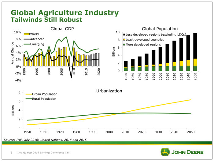
I would begin with a bit of context that might be useful as we ponder the outlook. Slide 1 shows the strong tailwinds that now drive the global agricultural economy. Major changes in agriculture and food markets began occurring sometime around the turn of the century and that ushered in a dozen or so unparalleled years characterized by strong demand growth, record high prices in farm incomes, food price spikes, expanded investment and innovation and increased trade.

A convergence of forces was responsible. These included global population growth, widespread global economic growth especially in emerging markets and developing countries, rapid urbanization and biofuels.

In 2000, the UN was projecting that the population would grow from 6.1 billion in that year to 9.3 billion by 2050. Today that projection for 2050 is 9.7 billion, so that’s another 2.4 billion from today’s 7.3 billion people.

Although having slowed somewhat, the global expansion continues especially across much of the developing world bringing millions more into the middle class and enabling ongoing improvements in diets.

On urbanization, we passed the 50% mark of population sometime around 2010 and that is now expected to approach 70% by 2050 with implications for food production and trade.

Slide 2 reflects global Ag as a whole showing the production and consumption of all global grains. Perhaps the most noteworthy point of this slide, and one often overlooked with all the focus on supply, acreage and yields, is the persistent consumption growth.

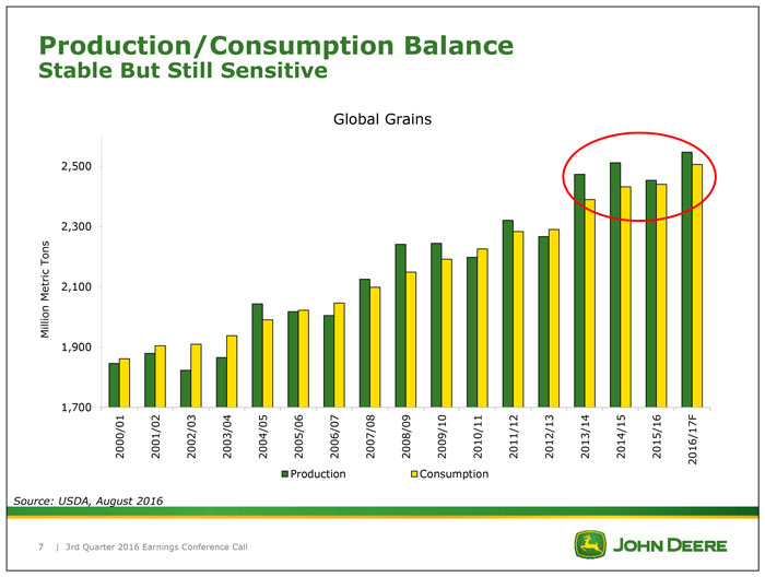
Consumption remains very strong, still rising steadily year-after-year and it has risen without fail every year since 1994-95, which included the great recession of 2009. Fueled by earlier high prices and after 4 consecutive great growing seasons worldwide, commodity supplies are now fully adequate to meet all needs. Prices, of course, have moved off their previously high levels and farmer margins have narrowed.

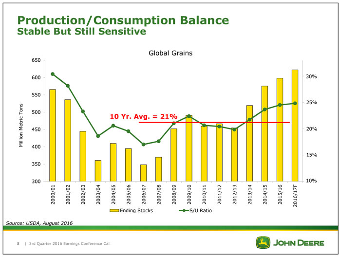
Slide 3 provides more details showing global stockholdings and the supply-to-use ratio. While carryover stocks (physical quantities) have reached levels of 15 years ago, it is important to remember that we are now consuming one-third more grains, so the supply-use ratio is the key indicator. While it has moved above the average of recent years, it remains in a sensitive area and especially so when viewed with Chinese grain stocks excluded. Notably the Chinese are thought to hold about 45% of the global stocks and the supply-use ratio actually has ticked down the last couple of years when the Chinese stocks are excluded.

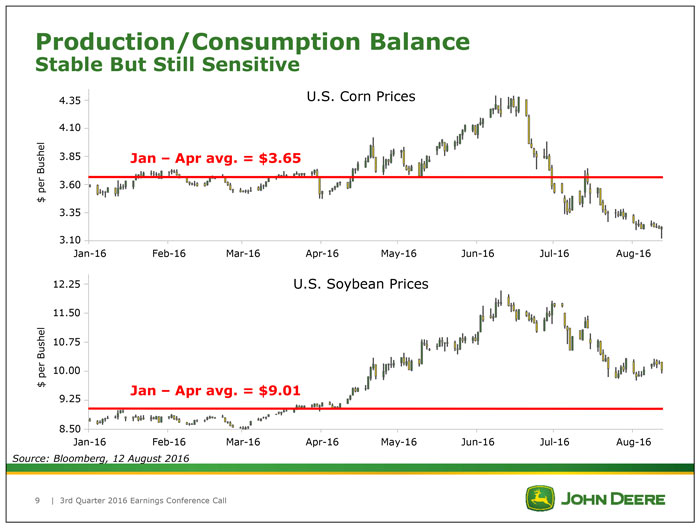
Slide 4 illustrates that even with abundant supply, the production-consumption balance still can shift rather quickly. Any significant production disruption will tilt the supply-use ratio downward and prices will immediately move higher. The recent price movements in response to reports of relatively minor weather events certainly highlighted continued sensitivity.

You will note from the slide that both corn and soybean futures were trading in a rather narrow range in the first 4 months of this year. Then we saw some reports of adverse weather in Brazil and Argentina in April  and prices quickly reflected the uncertainty it brought. Corn moved almost $0.90 bushel higher, soy moved $3.25 a bushel higher that's an increase of 25% for corn, 36% for soybeans.

Then by late June, the South American weather conditions abated followed by the early July USDA WASDE report, indicating larger acreages of both corn and soy. The weather premium quickly disappeared from the corn price and it was reduced per soybeans.

Just for reference, the U.S. drought in 2012 reduced corn yields 22% below trend pushing ending stocks to barely 800 million bushels and prices to new record high. But this year a corn yield reduction of only 4% would have been sufficient to reduce ending stocks to 1 billion bushels and push prices $5 per bushel or higher, a further illustration of the sensitive supply utilization balance. There was some expectation that farmers would reduce acreage in response to the softer prices as we came into the Northern Hemisphere planting seasons.

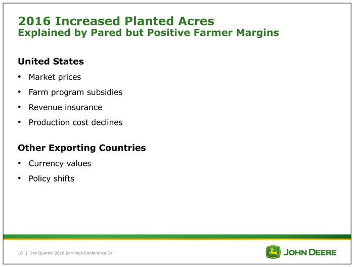
On Slide 5, we know that despite the softer prices, farmers worldwide did not reduce acreage. In the United States, farmer supply response this year was influenced by market prices, which provided a paired, but still positive margin. But they were also influenced by farm program subsidies, revenue insurance and production cost declines.

For example, the agricultural program ARC County forecast of 2015 payments for Illinois is $0.37 per bushel on corn-based acres and $0.98 per bushel on soybean based acres. So as a result of this combination, U.S. farmers this year expanded planted area for all major crops except wheat illustrating continued profitability despite softer prices.

Now we also expected a similar reduction in other parts of the world, but we noted there that farmers supply response was influenced largely by currency values and also some policy shifts, notably in Argentina. And in this crop year, major exporters expanded grain and oilseed area all around the world and grains and oilseeds were up 3.7% in South America.

For example, Brazilian farmers saw corn prices in reals of $5.24 per bushel in September 2015 compared to $3.43 per bushel a year before indicating that it was still very profitable to continue to expand.

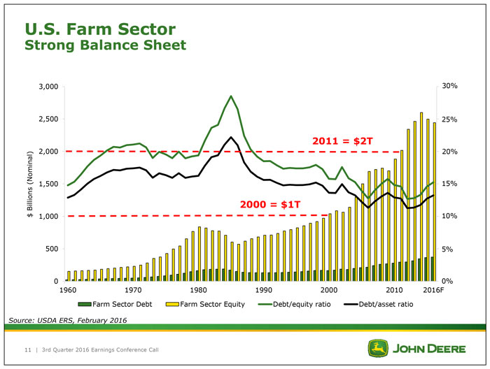
Slide 6 speaks to the financial condition of the U.S. farm sector. Overall, the farm sector balance sheet remains strong. Farmer debt has been well managed. The financial indicators are still solid. It was not until 2000 that farm sector equity reached $1 trillion, but then it took only 10 more years to add the second trillion dollars and 5 years later we have added another $0.5 trillion.

A major part of that balance sheet, of course, is farmland and USDA forecasts land prices to decline in 2016, cropland to decline 1%. This is the first time since 2009 and only the second time in almost 3 decades.

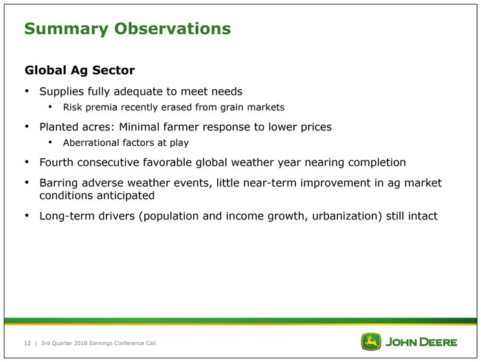
Slide 7 summarizes the situation across the global Ag sector. As I noted, supplies are fully adequate, the risk premium has been erased from the grain market. We saw very little reduction coming into the year in response to the lower prices and that was because of the aberrational forces at play — the subsidies, the risk measures and currency values, which boosted commodity prices and we're in the fourth consecutive favorable weather year.

So adding all of those things together barring adverse weather events, little near-term improvement in ag market conditions is anticipated, but we would note that the long-term drivers, population growth, income growth and urbanization are still intact.

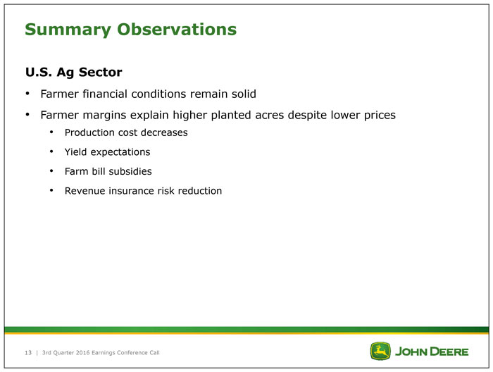
Slide 8 pertains to the U.S. ag sector and we note that farming is still profitable despite softer prices as evidenced by the continued expansion of planted acres this year and financial conditions across the sector remain solid. There is some individual farmer stress to be sure, but no widespread stress is yet evident.

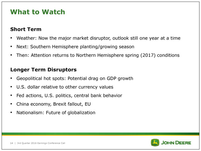
Slide 9 lists some key factors that are worth watching in the coming months. In the short term, weather is key. We know that demand is strong. We now know that supply depends upon the weather, so weather is still the major market disruptor and it's still one season at a time.

Attention now will turn from North America to the southern hemisphere as the planting/growing season gets underway there in late September and October. We’ll continue to watch that until next spring in the northern hemisphere when we start focusing on planting and growing conditions here. Over the longer term, I would note that any of these geopolitical hotspots that could erupt and become a drag on global GDP would be a negative.

Lots of other things to watch include relative currency values and the political situation in several countries, central bank behavior all over the world and so I would just conclude by noting that after a dozen years of unprecedented prosperity, planting, commodity prices, food prices and trading patterns are now stabilizing. A new commodity price trading range with favorable weather is emerging and weather remains the major commodity market disruptor. The outlook is still one year at a time depending upon the weather.